- Support Vector Machine(SVM)

The objective of the support vector machine algorithm is to find a hyperplane in an N-dimensional space that distinctly classifies the data points when given the dichotomous data .
Support vectors are data points that are closer to the hyperplane and influence the position and orientation of the hyperplane. Using these support vectors, we maximize the margin of the classifier. Deleting the support vectors will change the position of the hyperplane.
- The goal of SVM
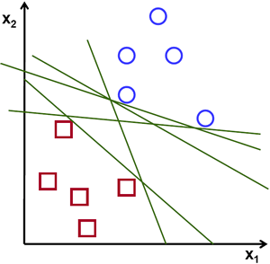
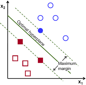
Our objective is to find a plane that has the maximum margin, i.e the maximum distance between data points of both classes. Maximizing the margin distance provides some reinforcement so that future data points can be classified with more confidence.
- Hyperplanes
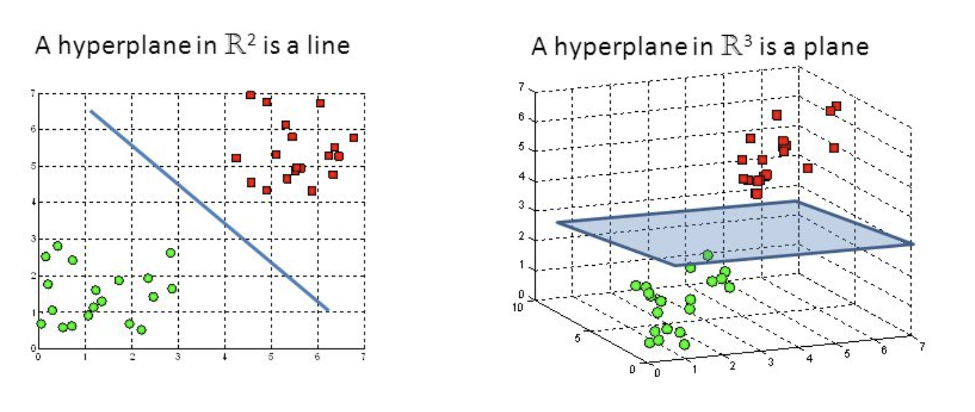
- Hyperplanes are decision boundaries that help classify the data points. Data points falling on either side of the hyperplane can be attributed to different classes.
- The dimension of the hyperplane depends upon the number of features. If the number of input features is 2, then the hyperplane is just a line. If the number of input features is 3, then the hyperplane becomes a two-dimensional plane.
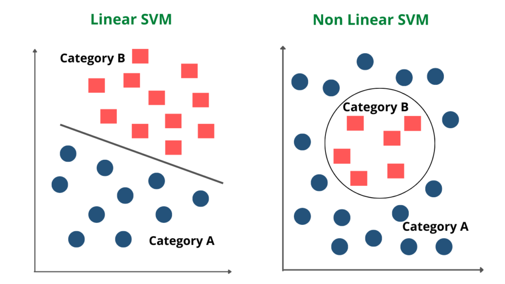
- Linear SVM VS Non Linear SVM
https://m.blog.naver.com/winddori2002/221662413641
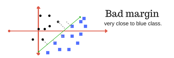
- Margin
The maximum distance between data points of both classes meaning maximize the margin between the data points and the hyperplane. Maximizing the margin distance provides some reinforcement so that future data points can be classified with more confidence.
reference : medium.com/machine-learning-101/chapter-2-svm-support-vector-machine-theory-f0812effc72

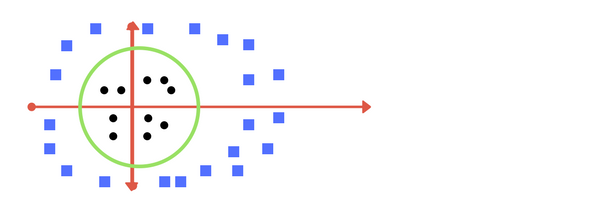
- Kernel
The hyperplace maps to circular boundary.
f(x) = B(0) + sum(ai * (x,xi))
For example, the inner product of the vectors [2, 3] and [5, 6] is 2*5 + 3*6 or 28
x=[2,3], xi=[5,6], the coefficients B0 and ai (for each input) must be estimated from the training data by the learning algorithm.
- Regularization(C)
It tells how much you want to avoid misclassifying each training example.
- Large value of C : The optimization will choose a smaller-margin hyperplane if that hyperplane does a better job of getting all the training points classified correctly
- Small value of C : The optimization will choose a larger-margin, even if thathyperplane misclassifies more points.


reference : www.analyticsvidhya.com/blog/2017/09/understaing-support-vector-machine-example-code/
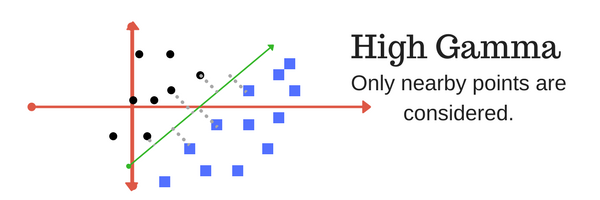
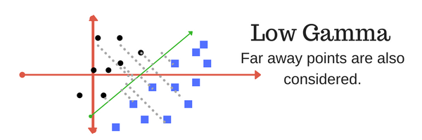
- Gamma
It defines how far the influence of a single training example reaches. Kernel coefficient for ‘rbf’, ‘poly’ and ‘sigmoid’.
- Higher gamma : It will try to exact fit training data set, it might cause over-fitting problem. Close points are considered.
- Lower gamma : Far points are also considered.

import numpy as np
import matplotlib.pyplot as plt
from sklearn import svm, datasets

iris=datasets.load_iris()
X=iris.data[:,:2]
y=iris.target
svc=svm.SVC(kernel='linear',C=1).fit(X,y)
x_min, x_max=X[:,0].min()-1, X[:,0].max()+1
x_min, x_max
>>>
(3.3, 8.9)

y_min,y_max=X[:,1].min()-1, X[:1].max()+1
y_min,y_max
>>>
(1.0, 6.1)

h=(x_max/x_min)/100
xx,yy=np.meshgrid(np.arange(x_min,x_max,h),np.arange(y_min,y_max,h))
plt.subplot(1,1,1)
Z=svc.predict(np.c_[xx.ravel(),yy.ravel()])
Z=Z.reshape(xx.shape)
plt.contourf(xx,yy,Z,cmap=plt.cm.Paired, alpha=0.8)

plt.scatter(X[:,0],X[:,1],c=y,cmap=plt.cm.Paired)
plt.xlim(xx.min(),xx.max())
plt.show()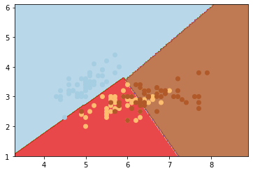
svm.SVC : Support Vector Machine.Support Vector Classification
- kernel : it has linear, rbf(Radial Basis Function), poly, default is 'rbf'.
- C : Classification, float, default=1.0
numpy.meshgrid : Return coordinate matrices from coordinate vectors.
- x1, x2, ..., xn : 1-D arrays representing the coordinates of a grid
matplotlib.subplot() : It creates a fifures and a grid of subplots with a single call.
- subplots() : without arguments returns a fiture and a single axes.
- subplots(2) : vertically stacked subplots
- subplots(1,2) : horizontally stacked subplots
SupportVectorMachin.predict() : after being fitted, the model can then be used to predict new values
numpy.ravel() : Return a contiguous flattened array.
x=np.array([[1,2,3],[4,5,6]])
x
>>>
array([[1, 2, 3],
       [4, 5, 6]])

np.ravel(x)
>>>
array([1, 2, 3, 4, 5, 6])
numpy.c_[] : Concatenation, translates slice objects to concatenation along the second axis.
np.c_[np.array([1,2,3]),np.array([4,5,6])]
>>>
array([[1, 4],
       [2, 5],
       [3, 6]])
numpy.reshape() : Gives a new shape to an array
x=np.array([[1,2,3],[4,5,6]])
np.reshape(x,(2,-1)) # -1 is inferred to be 2
>>>
array([[1, 2, 3],
       [4, 5, 6]])
matplotlib.pyplot.contourf() : Contour Filled
- cmap : ColorMap, str, default is rcParams, it maps the level values to colors. ('Pastel1', 'Pastel2', 'Paired', 'Accent', 'Dark2', 'Set1', 'Set2', 'Set3', 'tab10', 'tab20', 'tab20b', 'tab20c')
- alpha : float, default is 1, between 0(transparent) and 1(opaque)
matplotlib.pyplot.scatter()
- c : Color, array-like or list of colors
matplotlib.pyplot.xlim() : x Limits, get or set the x limits of the current axes
svc_rbf=svm.SVC(kernel='rbf',C=1,gamma=1).fit(X,y)
plt.subplot(1,1,1)
Z=svc_rbf.predict(np.c_[xx.ravel(),yy.ravel()])
Z=Z.reshape(xx.shape)
plt.contourf(xx,yy,Z,cmap=plt.cm.Paired, alpha=0.8)

plt.scatter(X[:,0],X[:,1],c=y,cmap=plt.cm.Paired)
plt.xlim(xx.min(),xx.max())
plt.show()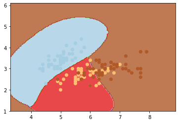
'Machine Learning' 카테고리의 다른 글
| Glance ML (0) | 2022.03.11 |
|---|---|
| Entropy, Cross-Entropy (0) | 2021.03.31 |
| Softmax (0) | 2021.03.24 |
| Logistic Regression, Sigmoid function (0) | 2021.03.17 |
| Scalar vs Vector vs Matrix vs Tensor (0) | 2021.03.17 |