- Logistic Regression
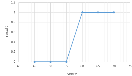
The problem that determines one of the two is called binary classification. And there is logistic regression for solving binary classification. It has a single layer of weights.
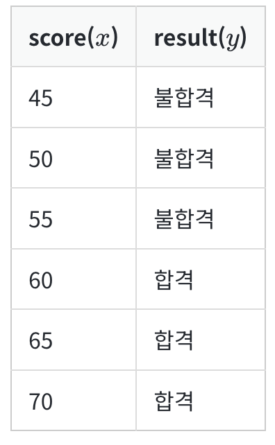
| x : given data y : result of x If result(y) has given, what result H(x) will get? |
- Sigmoid function
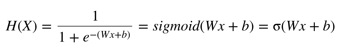 e(Euler's number)=2.718281... |
 Less than 0.5 is considered 0 More than 0.5 is considered 1 |
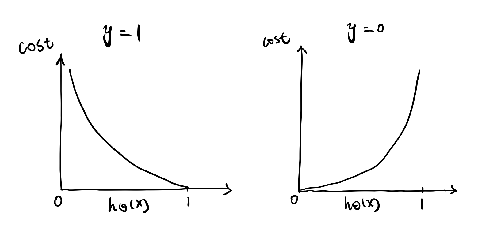
If y(result) is 1, the prediction is 1, then the cost is 0.
If y(result) is 1, the prediction is 0, then this is totally opposite prediction, so the learning algorithm is punished by a very large cost.
Vice versa.
Reference : towardsdatascience.com/optimization-loss-function-under-the-hood-part-ii-d20a239cde11
1. If W=1, b=0 (original : σ(Wx+b))
%matplotlib inline
import numpy as np
import matplotlib.pyplot as plt

def sigmoid(x):
  return 1/(1+np.exp(-x))
x = np.arange(-5.0, 5.0, 0.1)
y=sigmoid(x)

plt.plot(x,y,'g')
plt.plot([0,0],[1.0,0.0],':')
plt.show()
As a result, sigmoid turns out between 0 and 1
If x=0, σ(sigmoid)=0.5
If x increasing, it converges to 0
2. If W=0.5, 1, 2, b=0
def sigmoid(x):
  return 1/(1+np.exp(-x))
x=np.arange(-5.0,5.0,0.1)
y1=sigmoid(0.5*x)
y2=sigmoid(x)
y3=sigmoid(2*x)

plt.plot(x,y1, 'r', linestyle='--')
plt.plot(x,y2,'g')
plt.plot(x,y3,linestyle='--')
plt.plot([0,0],[1.0,0.0],':')
plt.show()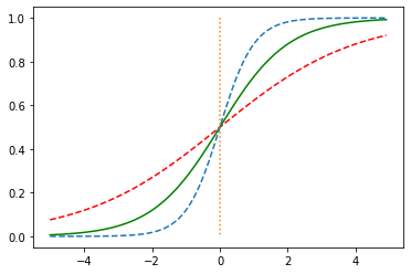
W meaning slope.
Increasing W, steeper slope. Vice versa.
3. If W=1, b=0.5, 1, 2
def sigmoid(x):
  return 1/(1+np.exp(-x))
x=np.arange(-5.0,5.0,0.1)
y1=sigmoid(x+0.5)
y2=sigmoid(x+1)
y3=sigmoid(x+1.5)

plt.plot(x,y1, 'r', linestyle='--')
plt.plot(x,y2,'g')
plt.plot(x,y3,linestyle='--')
plt.plot([0,0],[1.0,0.0],':')
plt.show()
4. Simple Logistic Regression
Hypothesis : y is 1 if x is over 10, otherwise y is 0.
import numpy as np
%matplotlib inline
import matplotlib.pyplot as plt
from tensorflow.keras.models import Sequential
from tensorflow.keras.layers import Dense
from tensorflow.keras import optimizers

X=np.array([-50, -40, -30, -20, -10, -5, 0, 5, 10, 20, 30, 40, 50])
y=np.array([0, 0, 0, 0, 0, 0, 0, 0, 1, 1, 1, 1, 1])

model=Sequential()
model.add(Dense(1,input_dim=1, activation='sigmoid'))

opt=optimizers.SGD(lr=0.01)
model.compile(optimizer=opt, loss='binary_crossentropy', metrics=['binary_accuracy'])
model.fit(X,y,batch_size=1, epochs=30, shuffle=False)
>>>
...

Epoch 29/30
13/13 [==============================] - 0s 1ms/step - loss: 0.1125 - binary_accuracy: 0.9526
Epoch 30/30
13/13 [==============================] - 0s 2ms/step - loss: 0.1117 - binary_accuracy: 0.9526

plt.plot(X,model.predict(X), 'b', X,y,'k.')

model.predict([1,2,3,4,5,10,11,12,13,14])
>>>
array([[0.45559546],
       [0.5141264 ],
       [0.57227236],
       [0.6284881 ],
       [0.6814285 ],
       [0.87362355],
       [0.89733815],
       [0.9170253 ],
       [0.9332182 ],
       [0.9464355 ]], dtype=float32)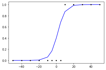
5. Multiple Logistic Regression
Hypothesis : y is 0 if x is 0, otherwise 1 if there is 1 in x.
X=np.array([[0,0],[0,1],[1,0],[1,1]])
y=np.array([0,1,1,1])

from tensorflow.keras.models import Sequential
from tensorflow.keras.layers import Dense
from tensorflow.keras import optimizers

model=Sequential()
model.add(Dense(1, input_dim=2, activation='sigmoid'))
model.compile(optimizer='sgd',loss='binary_crossentropy', metrics=['binary_accuracy'])
model.fit(X,y,batch_size=1, epochs=40, shuffle=False)
>>>
...
4/4 [==============================] - 0s 3ms/step - loss: 0.5540 - binary_accuracy: 0.5333
Epoch 400/400
4/4 [==============================] - 0s 2ms/step - loss: 0.5534 - binary_accuracy: 0.5333

model.predict(X)
>>>
array([[0.626424  ],
       [0.8194542 ],
       [0.82448316],
       [0.9270863 ]], dtype=float32)
Ecxept for [0,0], rest of pairs got close to 1.
'Machine Learning' 카테고리의 다른 글
| Entropy, Cross-Entropy (0) | 2021.03.31 |
|---|---|
| Support Vector Machine, Margin, Kernel, Regularization, Gamma (0) | 2021.03.30 |
| Softmax (0) | 2021.03.24 |
| Scalar vs Vector vs Matrix vs Tensor (0) | 2021.03.17 |
| Linear Regression, Simple Linear Regression, Multiple Linear Regression, MSE, Cost function, Loss function, Objective function, Optimizer, Gradient Descent (0) | 2021.03.16 |