2. DataFrame
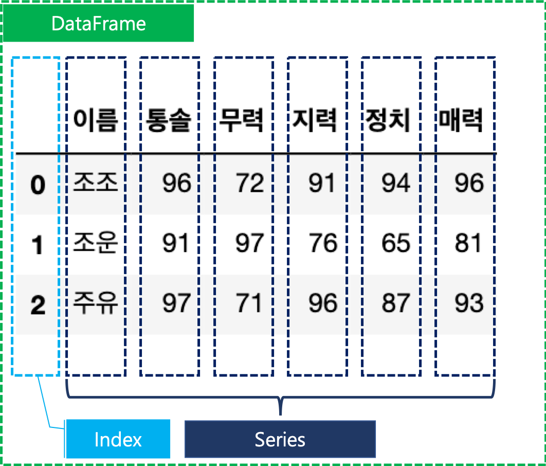
Two-dimensional, added columns to Series.
df=pd.DataFrame([[1,2,3],[4,5,6],[7,8,9]],index=['one','two','three'],columns=['a','b','c'])
df

>>>	a	b	c
one	1	2	3
two	4	5	6
three	7	8	9

df.values
>>>array([[1, 2, 3],
       [4, 5, 6],
       [7, 8, 9]])

df.index
>>>Index(['one', 'two', 'three'], dtype='object')

df.columns
>>>Index(['a', 'b', 'c'], dtype='object')
- Create DataFrame with list
data=[['1000', 'Steve', 90.72],
    ['1001', 'James', 78.09],
    ['1002', 'Doyeon', 98.43],
    ['1003', 'Jane', 64.19],
    ['1004', 'Pilwoong', 81.30],
    ['1005', 'Tony', 99.14]]

df=pd.DataFrame(data, index=['one','two','three','one','two','three'],columns=['a','b','c'])
df
>>>	a	b	c
one	1000	Steve	90.72
two	1001	James	78.09
three	1002	Doyeon	98.43
one	1003	Jane	64.19
two	1004	Pilwoong	81.30
three	1005	Tony	99.14
- Create DataFrame with dictionary
data={'a':['1000', '1001', '1002', '1003', '1004', '1005'],
      'b':['Steve', 'James', 'Doyeon', 'Jane', 'Pilwoong', 'Tony'],
      'c':[90.72, 78.09, 98.43, 64.19, 81.30, 99.14]}
df=pd.DataFrame(data,index=['one','two','three','one','two','three'])
df
>>>	a	b	c
one	1000	Steve	90.72
two	1001	James	78.09
three	1002	Doyeon	98.43
one	1003	Jane	64.19
two	1004	Pilwoong	81.30
three	1005	Tony	99.14
pd.DataFrame({
'class':['a','b','c'],
'val1':(np.random.rand(3)*100).astype(int),
'val2':(np.random.rand(3)*100).astype(int),
'val3':(np.random.rand(3)*100).astype(int)
})
>>>
class val1 val2 val3
0 a 38 80 1
1 b 79 85 44
2 c 90 1 44
- loc
Location, access a group of rows using with index name.
c2=pd.DataFrame(data,index=['A', 'B', 'C','A', 'B', 'C'])
c2
a	b	c
A	1000	Steve	90.72
B	1001	James	78.09
C	1002	Doyeon	98.43
A	1003	Jane	64.19
B	1004	Pilwoong	81.30
C	1005	Tony	99.14

c2.loc[['A','C']]
a	b	c
A	1000	Steve	90.72
A	1003	Jane	64.19
C	1002	Doyeon	98.43
C	1005	Tony	99.14
Set value. For example,
df.loc[item1,item2]=10 : Find item1 and put 10 to item2 of item1.
df.loc[['viper', 'sidewinder'], ['shield']] = 50

>>>
df

            max_speed  shield
cobra               1       2
viper               4      50
sidewinder          7      50
df.loc[item1,item2]=100 : Find item1 and create item2, and then put 100 to item2.
df.loc[df.index, 'abc']=100

>>>

	    max_speed	shield	abc
cobra	      1	         2     100.0
viper	      4	         5     100.0
sidewinder    7	         8     100.0
- iloc
Integer Location, access a group of rows using with index number.
df
>>>
	a	b	c	d
0	1	2	3	4
1	100	200	300	400
2	1000	2000	3000	4000

df.iloc[0,2]
>>>
3

df.iloc[[0,2]]
>>>
a	b	c	d
0	1	2	3	4
2	1000	2000	3000	4000
- at
Access a single value for a row/column label pair.
c2.at['A','b']
A    Steve
A     Jane
Name: b, dtype: object
- isin
DataFrame.isin() : Is () in DataFrame? Return dataframe if yes.
c2[c2['c'].isin([90.72])]
a	b	c
A	1000	Steve	90.72
- drop
Drop specified labels from rows or columns.
- axis=1 : Drop the column
- axis=0 : Drop the row
lst_df.drop(columns=['new'])
- astype
DataFrame.astype() : Change the DataFrame type as ()
c2['c'].astype('int')
A    90
B    78
C    98
A    64
B    81
C    99
Name: c, dtype: int64
- .astype('category') : Data can be categorized
train=pd.read_csv("https://raw.githubusercontent.com/developer-sdk/kaggle-python-beginner/master/datas/kaggle-titanic/train.csv")
train['SexCate']=train['Sex'].astype('category')
- cut
It used when you need to segment and sort data values into bins.
- labels : Specifies the labels for the returned bins. Must be the same length as the resulting bins.
pd.cut(train['Age'],3,labels=['young','mid','old'])
>>>
0      young
1        mid
2      young
3        mid
4        mid
       ...
886      mid
887    young
888      NaN
889    young
890      mid
Name: Age, Length: 891, dtype: category
Categories (3, object): ['young' < 'mid' < 'old']
- bins : It values into discrete intervals. It should be one more than number of labels.
pd.cut(train['Fare'],bins=[-1, 0, 8, 15, 32, 100, 600],labels=[1, 2, 3, 4, 5, 6])
0      2
1      5
2      2
3      5
4      3
      ..
886    3
887    4
888    4
889    4
890    2
Name: Fare, Length: 891, dtype: category
Categories (6, int64): [1 < 2 < 3 < 4 < 5 < 6]
- qcut
qcut(DataFrame, 10) : Discrete DataFrame to 10 as same size.
Quantile cut, it discretes same size.
pd.qcut(train['Fare'],10)
0        (-0.001, 7.55]
1      (39.688, 77.958]
2         (7.854, 8.05]
3      (39.688, 77.958]
4         (7.854, 8.05]
             ...
886      (10.5, 14.454]
887      (27.0, 39.688]
888      (21.679, 27.0]
889      (27.0, 39.688]
890       (7.55, 7.854]
Name: Fare, Length: 891, dtype: category
Categories (10, interval[float64]): [(-0.001, 7.55] < (7.55, 7.854] < (7.854, 8.05] < (8.05, 10.5] ... (21.679, 27.0] < (27.0, 39.688] < (39.688, 77.958] < (77.958, 512.329]]
- factorize
The values can be changed to integer.
df = pd.DataFrame({"A":["a", "b", "c", "a", "d"]})
df.A = df.A.astype('category')
codes, uniques = pd.factorize(df.A)
pd.factorize(df.A)
>>>
(array([0, 1, 2, 0, 3]),
 CategoricalIndex(['a', 'b', 'c', 'd'], categories=['a', 'b', 'c', 'd'], ordered=False, dtype='category'))

pd.factorize(df.A)[0]
>>>
array([0, 1, 2, 0, 3])

pd.factorize(df.A)[1]
>>>
CategoricalIndex(['a', 'b', 'c', 'd'], categories=['a', 'b', 'c', 'd'], ordered=False, dtype='category')
- sort_index
- ascending=True : ascending order, False is descending order
- sort_values
- by='column' : Align the values by column
- ascending : Sort ascending, derault True
df=pd.DataFrame({'col1':['A', 'A', 'B', np.nan, 'D', 'C'],'col2':['a', 'B', 'c', 'D', 'e', 'F'],'col3':[2, 1, 9, 8, 7, 4]})
df
>>>
	col1	col2	col3
0	A	a	2
1	A	B	1
2	B	c	9
3	NaN	D	8
4	D	e	7
5	C	F	4

df.sort_values(by=['col2','col3'])
>>>
col1	col2	col3
1	A	B	1
3	NaN	D	8
5	C	F	4
0	A	a	2
2	B	c	9
4	D	e	7
total_bill tip sex smoker day time size
0 16.99 1.01 Female No Sun Dinner 2
1 10.34 1.66 Male No Sun Dinner 3
2 21.01 3.50 Male No Sun Dinner 3
df.sort_values(by=['total_bill', 'tip'],ascending=[True, False])
###### Sort the data with multiple columns in different directions ######
- iterrows
Iterate over DataFrame rows as index, Series pairs.
df = pd.DataFrame({
    '이름': ['조조', '조운', '주유'],
    '통솔': [96, 91, 97],
    '무력': [78, 97, 71],
    '지력': [91, 28, 96],
    '정치': [94, 78, 87],
    '매력': [96, 81, 87]
})

>>>

	이름	통솔	무력	지력	정치	매력
0	조조	96	78	91	94	96
1	조운	91	97	28	78	81
2	주유	97	71	96	87	87

for index,row in df.iterrows():
    print(index)
>>>
0
1
2

for index,row in df.iterrows():
    print(row)
>>>
이름    조조
통솔    96
무력    78
지력    91
정치    94
매력    96
Name: 0, dtype: object
이름    조운
통솔    91
무력    97
지력    28
정치    78
매력    81
Name: 1, dtype: object
이름    주유
통솔    97
무력    71
지력    96
정치    87
매력    87
Name: 2, dtype: object
- itertuple
Iterate over DataFrame rows as named tuples
for index in df.itertuples():
    print(index)

Pandas(Index=0, 이름='조조', 통솔=96, 무력=78, 지력=91, 정치=94, 매력=96)
Pandas(Index=1, 이름='조운', 통솔=91, 무력=97, 지력=28, 정치=78, 매력=81)
Pandas(Index=2, 이름='주유', 통솔=97, 무력=71, 지력=96, 정치=87, 매력=87)
- groupby
Grouping the DataFrame by column.
df=pd.DataFrame({
    'class':[['A','B','C'][np.random.randint(0,3)] for i in range(0,10)],
    'year':[['2019','2020'][np.random.randint(0,2)] for i in range(0,10)],
    'month':[np.random.randint(5,7) for i in range(0,10)],
    'val1':[np.random.randint(10000,20000) for i in range(0,10)],
    'val2':[np.random.randint(100,300) for i in range(0,10)],
    'val3':[np.random.randint(1,11) for i in range(0,10)]
    })

classgroup=df.groupby(['class','year']).count()
classgroup
			month	val1	val2	val3
class	year
	A	2019	2	2	2	2
		2020	3	3	3	3
	B	2020	1	1	1	1
	C	2019	1	1	1	1
		2020	3	3	3	3
remainder=df.groupby(lambda x:x//2)
remainder.sum()
month val1 val2 val3
0 11 34223 428 12
1 12 30678 368 9
2 12 27858 374 11
3 10 26259 280 16
4 11 27201 430 8
- agg
Aggregate
classgroup.agg(['max','min'])

	month	val1	val2	val3
max	3	3	3	3
min	1	1	1	1
remainder.agg({'val1':'min','val2':'max','val3':['min','max']})
val1 val2 val3
min max min max
0 17018 270 2 10
1 14071 222 4 5
2 12782 239 1 10
3 11640 149 8 8
4 10807 233 3 5
- crosstab
Cross Tabulation, compute a simple cross tabulation of two or more factors.
- margins=True : Show subtotals.
pd.crosstab(train['Sex'],train['SexCate'],margins=True)

SexCate	female	male	All
Sex
female	314	0	314
male	0	577	577
All	314	577	891
-values : Array of values to aggregate to the factors. Requires affgunc be specified.
- aggfunc : Aggregate Function
pd.crosstab(train['Sex'],train['Age'],values=train['Survived'], aggfunc=sum)

Age	young	mid	old
Sex
female	126	95	12
male	56	49	4
- concat
Concatenate
- ignore_index=True : Do not use the index values along the concatenation axis.
s1=pd.Series(['a','b'])
s2=pd.Series(['c','d'])
pd.concat([s1,s2])
>>>
0    a
1    b
0    c
1    d
dtype: object

s1=pd.Series(['a','b'])
s2=pd.Series(['c','d'])
pd.concat([s1,s2],ignore_index=True)
>>>
0    a
1    b
2    c
3    d
dtype: object
- join='inner' : Join the column under the same name, default is 'outer'
s1=pd.DataFrame({'col1':['a','b'],'col2':[1,2]})
s2=pd.DataFrame({'col2':['c','d'],'col3':[3,4]})
pd.concat([s1,s2],ignore_index=True)

>>>

      col1	 col2     col3
0	a	  1	   NaN
1	b	  2	   NaN
2	NaN	  c	   3.0
3	NaN	  d	   4.0

pd.concat([s1,s2],ignore_index=True, sort=False, join='inner')

>>>

      col2
0	1
1	2
2	c
3	d
- style
- merge
- on : These must be found in both DataFrames and merging to the intersection of the columns in both DataFrames.
df1 = pd.DataFrame({'lkey': ['foo', 'bar', 'baz', 'foo'],
                    'value': [1, 2, 3, 5]})
df2 = pd.DataFrame({'rkey': ['foo', 'bar', 'baz', 'foo'],
                    'value': [5, 1, 7, 8]})
print(df1)
print('------')
print(df2)
>>>
  lkey  value
0  foo      1
1  bar      2
2  baz      3
3  foo      5
------
  rkey  value
0  foo      5
1  bar      1
2  baz      7
3  foo      8

combined=pd.merge(df1,df2,on='value')
combined
>>>
lkey	value	rkey
0	foo	1	bar
1	foo	5	foo
- pivot_table
Create a spreadsheet-style pivot table as a DataFrame.
dataframe.pivot_table(values=, index=, columns=, fill_value=)
- values : value supposed to insert to value
- index, columns : column
- fill_value : scalar, value to replace missing values with.
- aggfunc : Aggregate Function, it aggregates values by using the function.
rating_crosstab=combined_movies_data.pivot_table(values='rating', index='user_id', columns='movie title', fill_value=0)df=pd.DataFrame({'a':["foo", "foo", "foo", "foo", "foo"],'b':["one", "one", "one", "two", "two"],'c':["small", "large", "large", "small",
"small"],'d':[1, 2, 2, 3, 3]})
df
>>>
a b c d
0 foo one small 1
1 foo one large 2
2 foo one large 2
3 foo two small 3
4 foo two small 3
pd.pivot_table(df, values='d',index=['a','b'],columns=['c'],aggfunc=np.sum)
>>>
c large small
a b
foo one 4.0 1.0
two NaN 6.0
- get_loc
Get Location, slice or boolean mask for requested label.
a=pd.Index(list('abc'))
a.get_loc('b')
>>>
1
- corr_mat
Correlation matrix, returns a correlation matrix of a dataframe. Several different correlation methods can be choosen and the matrix can be created for column or row relations.
- sparse
You can view the object as being compressed where any data matching a specific value(NaN, missing value, though any value can be chosen, including 0) is omitted. The compressed values are not actually stored in the array.
arr=np.random.randn(10)
arr[2:-2]=np.nan
pd.Series(pd.arrays.SparseArray(arr))
>>>
0    0.256553
1    0.671573
2         NaN
3         NaN
4         NaN
5         NaN
6         NaN
7         NaN
8    0.582745
9    1.599741
dtype: Sparse[float64, nan]
- from_spmatrix
Sparse Matrix
- rename
Renaming columns of an existing DataFrame.
- inplace : If True, it will make changes on the original DataFrame.
data={'name':['John', 'Doe', 'Paul'],
      'age':[22, 31, 15]}
df=pd.DataFrame(data)
df.rename(columns={'name':'first name','age':'AGE'},inplace=True)
df
>>>
	first name	AGE
0	John	22
1	Doe	31
2	Paul	15
- values.tolist
Convert DataFrame value to List.
Inst_Att
INST_NM	DRULE_ATT_TYPE_CODE1
0	대구대학교	Attack
1	경기대학교	Attack

df_list=Inst_Att.values.tolist()
df_list
>>>
[['대구대학교', 'Attack'],
 ['경기대학교', 'Attack']]
- columns.tolist
Convert DataFrame columns to List.
0	1	2	3	4	mean
0	0.621096	0.904698	0.629040	0.109003	0.648523	0.325452


cols=df.columns.tolist()
cols
>>>
[0, 1, 2, 3, 4, 'mean']
- drop_duplicates
To get unique values of column, it removes all duplicated values and returns a Pandas series.
- explode
Transform each element of a list-like to a row.
df = pd.DataFrame({'A': [[0, 1, 2], 'foo', [], [3, 4]],
                   'B': 1,
                   'C': [['a', 'b', 'c'], np.nan, [], ['d', 'e']]})

df.explode('A')
>>>
     A  B          C
0    0  1  [a, b, c]
0    1  1  [a, b, c]
0    2  1  [a, b, c]
1  foo  1        NaN
2  NaN  1         []
3    3  1     [d, e]
3    4  1     [d, e]
- How to get column name
for col in df_100.columns:
  print(col)

>>>
TW_ATT_IP_SEARCH_DATA
TW_ATT_GEOLOCATION
ACCD_CHARGER_ID
...
- How to remove nan from all columns
for column_name in df.columns:
    df[column_name]=df[column_name].replace(np.nan, '')
- isna
Detect missing values.
NTM_df.isna().sum()

>>>
INST_NM                 0
DRULE_ATT_TYPE_CODE1    0
TW_ATT_IP               0
TW_ATT_PORT             0
TW_DMG_IP               0
TW_DMG_PORT             0
ACCD_DMG_PROTO_NM       1
- mean
Return the mean of the values over the requested axis.
- mean(0) : index
- mean(1) : columns
df['mean']=df.mean(1)
df
>>>
0	1	2	3	4	mean
0	0.279847	0.956025	0.030422	0.994737	0.129731	0.478152
1	0.186938	0.276841	0.011527	0.062197	0.761385	0.259778
- interpolate
Fill NaN values using an interpolation method.
-method='linear' : To guess the missing values and fill the data.
-limit_direction : Consecutive NaNs will be filled in this direction, default is ‘backward’. It indicates whether the missing values will be guessed using the previous values or latter values of the column.
https://pandas.pydata.org/docs/reference/api/pandas.DataFrame.interpolate.html
interpolate_df=cleaned_df.interpolate(method='linear',limit_direction='forward')
print(interpolate_df.isnull().any())
>>>
Category         False
Item             False
Calories         False
Total Fat        False
...
- query
Filter the data with easy way.
df.loc[(df['tip']>6) & (df['total_bill']>=30)]

>>>

	total_bill	tip	sex	smoker	day	time	size
23	39.42	7.58	Male	No	Sat	Dinner	4
59	48.27	6.73	Male	No	Sat	Dinner	4
141	34.30	6.70	Male	No	Thur	Lunch	6

###### Above is same as below ######

df.query("tip>6 & total_bill>=30")
- nunique
Count number of unique elements.
d1=pd.DataFrame({'a':[4,5,6],'b':[4,1,1]})
d1.nunique()

>>>

a    3
b    2
- size
Return the number after count.
d1=pd.DataFrame({'col1':[1,2],'col2':[2,3]})
d1.size

>>>
4
- reset_index
Reset the index.
drop=True : Drop the index column, default is False.
ex_df=pd.DataFrame(np.arange(0,9).reshape(3,3))
ex_df

>>>

	0	1	2
0	0	1	2
1	3	4	5
2	6	7	8

ex_df.reset_index()

>>>

	index	0	1	2
0	    0	0	1	2
1	    1	3	4	5
2	    2	6	7	8

ex_df.reset_index(drop=True)

>>>

	    0	1	2
0	    0	1	2
1	    3	4	5
2	    6	7	8
'Analyze Data > Python Libraries' 카테고리의 다른 글
| pandas-5. json_normalize (0) | 2021.10.25 |
|---|---|
| mlxtend-TransactionEncoder, association_rules (0) | 2021.06.23 |
| pandas-4. read_csv, unique, to_csv, file upload, file download (0) | 2021.06.22 |
| numpy-array, arange, reshape, slicing, newaxis, ...(Ellipsis) (0) | 2021.05.25 |
| pandas-1. Series, reindex, isnull, notnull, fillna, drop, dropna, randn, describe, nan, value_counts, map, apply, concat (0) | 2021.03.05 |