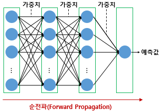
- Forward Propagation
Input layer-->hidden layer-->activation function-->output layer
--------------------------------------------------------------> in order
The input data is fed in the forward direction through the network. Each hidden layer accepts the input data, processes it as per the activation function and passes to the successive layer. In order to generate output, the input data should be fed in the forward direction only. The data should not flow in reverse direction during output generation otherwise it would form a cycle and the output could never be generated.
from keras.models import Sequential
from keras.layers import Dense
model=Sequential()
model.add(Dense(8,input_dim=4, init='uniform', activation='relu')) #4 input, 8 output
model.add(Dense(8,activation='relu')) #8 input, 8 output
model.add(Dense(3,activation='softmax')) #8 input, 3 output
					 #3 input, 3 output
- Optimizer
How much reduce the loss(find the most efficient W and b) is depends on which optimizer you are using.
1. Batch Gradient Descent
It considers entire data when seek the loss. It executes once entire parameter update per one epoch. Hence, it takes a long time but can seek the global minimum. It uses the whole training data to update weight and bias. Suppose if we have millions of records then training becomes slow and computationally very expensive.
model.fit(X_train, y_train, batch_size=len(train_X))
2. Stochastic Gradient Descent(SGD)
It solved the Batch Gradient Descent problem by using only single records to updates parameters.
model.fit(X_train, y_train, batch_size=1)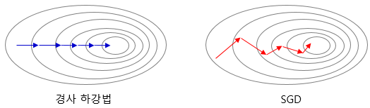
3. Mini Batch Gradient Descent
It overcomes the SGD drawbacks by using a designated data to update the parameter. Since it doesn't use entire records to update parameter, the path to reach global minima is not as smooth as Batch Gradient Descent. It updates the model parameters after every batch. So, the dataset is divided into various batches and after every batch, the parameters are updated.
model.fit(X_train, y_train, batch_size=32) #when it applys 32 as batch size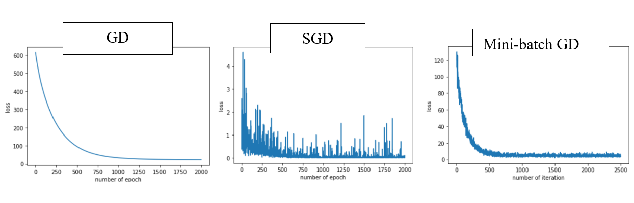
- reference : towardsdatascience.com/deep-learning-optimizers-436171c9e23f
4. Momentum
When cost reaches local minimum, the computation might recognize it reaches to global minimum, in this case, with momentum, it accelerates the convergence towards the relevant direction and reduces the fluctuation to the irrelevant direction, it helps get out of local minimum.
keras.optimizers.SGD(lr = 0.01, momentum= 0.9)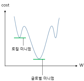
5. Adagrad
It changes the learning rate for each parameter and at every time step. Since constant learning rate for all parameters is not effeicient. It makes big updates for less frequent parameters and a small step for frequent parameters.
keras.optimizers.Adagrad(lr=0.01, epsilon=1e-6)- reference : towardsdatascience.com/optimizers-for-training-neural-network-59450d71caf6
6. Rprop
Resilient BackPropagation, it used for full-batch optimization. It combines the idea of only using the sign of the gradient with the idea of adapting the step size individually for each weight. Hence, the step size that's defined for that particular weight. And that step size adapts individually over time, so that we accelerate learning in the direction that we need.
7. RMSprop
Root Mean Square Propagation, with mini-batches, force the number we divide by to be similar for adjacent mini-batches rather than divide by different gradient every time. Hence, keep the moving average of the squared gradients for each weight. And then we divide the gradient by square root the men square.
When we have small learning rate, it averages the gradients over successive mini-batches. Consider the weight, that gets the gradient 0.1 on nine mini-batches, and the gradient of -0.9 on tenths mini-batch.
keras.optimizers.RMSprop(lr=0.001, rho=0.9, epsilon=1e-06)- reference : towardsdatascience.com/understanding-rmsprop-faster-neural-network-learning-62e116fcf29a
8. Adam
Adaptive Moment Estimation, works with momentums for both of direction and learning rate efficiency.
keras.optimizers.Adam(lr=0.001, beta_1=0.9, beta_2=0.999, epsilon=None, decay=0.0, amsgrad=False)
- Epoch
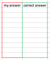
The machine is updating weight from error which comes from between prediction(y-hat, my answer) and real value(y, correct answer).
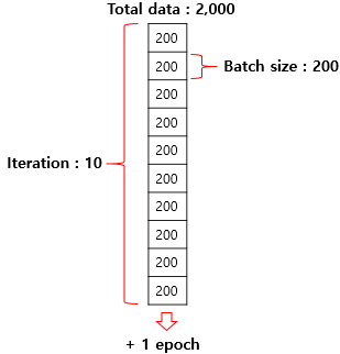
Epoch is the state that finished study for all the question comparing between my anwer and correct answer. For example, epoch is 50 meaning studied 50 times whole the question.
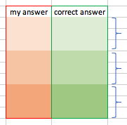
- Batch size
It is how many question I am going to check between my answer and correct answer, for example, I am going to check all the question and study again or per 10 questions or so on. If I am checking every 10 my answer with correct answer, the point to start to check between my answer and correct answer is the point update optimizer after compute the error. For example, per every 200 questions I am going to check among 2,000 questions, batch size is 200.
- Iteration
If whole the quesions is 2,000, and I am going to check my anwser with correct answer per every 200 questions, the number of iteration is 10, meaning the number of batch size in order to finish once epoch.